Getting started with Diffsky mocks

This notebook shows how to load diffsky data, and compute photometry and high-res SEDs.

Diffsky-native data format

The mock data natively produced by diffsky is stored as a collection of flat hdf5 files. Each hdf5 file has a name such as:

lc_cores-{stepnum}.{lc_patch}.diffsky_gals.hdf5,

where stepnum specifies the N-body simulation snapshot, and lc_patch specifies the patch of sky. Galaxies with the same stepnum occupy the same narrow range of redshift, and galaxies with the same lc_patch fall within the same contiguous patch of {ra, dec}.

The next cell shows how to load all the mock data stored in a single such file. (If you only need a subset of the columns, you can pass the keys keyward argument to the load_diffsky_lc_patch).

import numpy as np
from matplotlib import pyplot as plt

import os
drn_mock = "mock_download_dir"
bn_mock = "lc_cores-453.0.diffsky_gals.hdf5"
fn_mock = os.path.join(drn_mock, bn_mock)

from diffsky.data_loaders.hacc_utils import load_lc_mock as llcm
diffsky_lc_patch, metadata = llcm.load_diffsky_lc_patch(fn_mock)

OpenCosmo-formatted data

There are separate OpenCosmo-formatted data products that enable efficient querying and filtering with the OpenCosmo toolkit.

This notebook demonstrates how to load and analyze diffsky-native data. A separate OpenCosmo-based tutorial is coming soon.

Inspect the mock data

The diffsky_lc_patch dictionary stores every column of the mock, along with supplementary metadata needed to compute photometry.

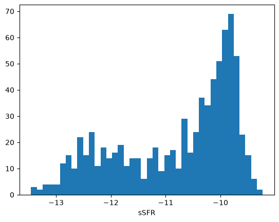
In this next cell we’ll take a look at a histogram of specific star formation rate, sSFR = log10(Mstar/SFR).

fig, ax = plt.subplots(1, 1)
__=ax.hist(diffsky_lc_patch['logssfr_obs'], bins=40)
xlabel = ax.set_xlabel('sSFR')

Examining mock photometry

The data stored in diffsky_lc_patch and metadata have all that is needed in order to recompute the photometry in the mock with the compute_phot_from_mock function. In the next few cells we’ll see how to recompute the photometry for a subset of the transmission curves used to make the mock.

The tcurves entry of metadata is a namedtuple that stores all of the transmission curves that were used to generate the mock photometry. You can see what bandpasses are present in the mock by inspecting the fields:

print(metadata['tcurves']._fields)

('lsst_u', 'lsst_g', 'lsst_r', 'lsst_i', 'lsst_z', 'lsst_y', 'roman_F062', 'roman_F087', 'roman_F106', 'roman_F129', 'roman_F158', 'roman_F184', 'roman_F146', 'roman_F213', 'roman_Prism', 'roman_Grism_1stOrder', 'roman_Grism_0thOrder')

For each bandpass, there is a corresponding column of mock data storing the photometry through that filter:

for bandpass_name in metadata['tcurves']._fields:
    assert bandpass_name in diffsky_lc_patch.keys()

Recomputing mock photometry

In the next few cells, we’ll recompute photometry through the lsst_u and lsst_i bands, and then compare the recomputed result to the corresponding columns of the mock.

Calculating photometry/SEDs in batches

Depending on your available computing resources, you may need to compute photometry for only a chunk of the data at a time to avoid overflowing memory.

Important note: Use the get_lc_mock_chunk function to grab a chunk of mock data. If you attempt to compute photometry or SEDs for an arbitrarily subdivided diffsky_lc_patch, you will get incorrect results, because the data chunk needs to have a complete set of satellite galaxies for each central.

batch_size = 20
nchunks = llcm.estimate_nchunks(fn_mock, batch_size)

chunknum = 0
diffsky_lc_patch_chunk = llcm.get_lc_mock_chunk(
    diffsky_lc_patch, metadata,
    nchunks=nchunks, chunknum=chunknum)

By default, the compute_phot_from_mock function assumes you want to recompute photometry through all available bands. You can use the tcurves argument to select a subset of transmission curves for which to compute photometry. In this next cell, we’ll pick just two bands: u and i, and show that our recomputed photometry agrees with the corresponding columns in the mock.

all_tcurves = metadata['tcurves']

from collections import namedtuple
Tcurves = namedtuple("Tcurves", ("lsst_u", "lsst_i"))
tcurves = Tcurves(all_tcurves.lsst_u, all_tcurves.lsst_i)

from diffsky.data_loaders.hacc_utils import sed_from_mock
phot_info = sed_from_mock.compute_phot_from_mock(
    diffsky_lc_patch_chunk, metadata, tcurves=tcurves
)

assert np.allclose(
    diffsky_lc_patch_chunk['lsst_u'],
    phot_info['obs_mags'][:, 0], rtol=1e-4)
assert np.allclose(
    diffsky_lc_patch_chunk['lsst_i'],
    phot_info['obs_mags'][:, 1], rtol=1e-4)

Recompute photometry of disk/bulge/knot decomposition

The photometry of each morphological component can be calculated using the compute_dbk_phot_from_diffsky_mock function.

dbk_phot_info, dbk_weights = sed_from_mock.compute_dbk_phot_from_mock(
    diffsky_lc_patch_chunk, metadata, tcurves=tcurves)

assert np.allclose(
    diffsky_lc_patch_chunk['lsst_u_bulge'],
    dbk_phot_info['obs_mags_bulge'][:, 0], rtol=1e-4)
assert np.allclose(
    diffsky_lc_patch_chunk['lsst_i_bulge'],
    dbk_phot_info['obs_mags_bulge'][:, 1], rtol=1e-4)

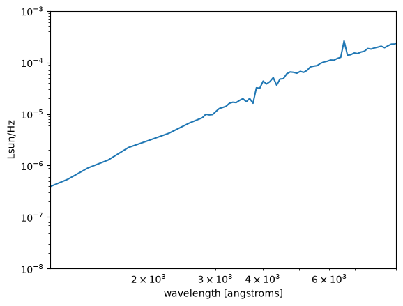
Compute SED of diffsky galaxies

There is also a convenience function for computing the high-resolution SED of each diffsky galaxy.

sed_info = sed_from_mock.compute_sed_from_mock(
    diffsky_lc_patch_chunk, metadata)

fig, ax = plt.subplots(1, 1)
__=ax.loglog()
xlim = ax.set_xlim(1_100, 9_000)
ylim = ax.set_ylim(1e-8, 1e-3)

igal = 5
__=ax.plot(metadata['ssp_data'].ssp_wave,
           sed_info['rest_sed'][igal, :])
xlabel = ax.set_xlabel('wavelength [angstroms]')
ylabel = ax.set_ylabel('Lsun/Hz')

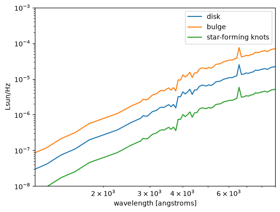
Compute SED of disk/bulge/knot components

There is an additional convenience function for computing the high-resolution SED of each morphological component.

dbk_sed_info = sed_from_mock.compute_dbk_sed_from_mock(
    diffsky_lc_patch_chunk, metadata)

fig, ax = plt.subplots(1, 1)
__=ax.loglog()
xlim = ax.set_xlim(1_100, 9_000)
ylim = ax.set_ylim(1e-8, 1e-3)

igal = 12
__=ax.plot(
    metadata['ssp_data'].ssp_wave,
    dbk_sed_info['rest_sed_disk'][igal, :], label='disk')
__=ax.plot(
    metadata['ssp_data'].ssp_wave,
    dbk_sed_info['rest_sed_bulge'][igal, :], label='bulge')
__=ax.plot(
    metadata['ssp_data'].ssp_wave,
    dbk_sed_info['rest_sed_knots'][igal, :], label='star-forming knots')
xlabel = ax.set_xlabel('wavelength [angstroms]')
ylabel = ax.set_ylabel('Lsun/Hz')
leg = ax.legend()

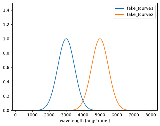
Computing photometry in other bands

You can compute photometry in other bandpasses by using the tcurves argument to store any sequence of transmission curves. Each individual transmission curve must be a namedtuple with two fields: wave and transmission; your sequence of transmission curves also needs to be formatted as a namedtuple, using whatever names you want to name each bandpass.

The next few cells show how to compute photometry through two arbitrary bandpasses.

from jax.scipy.stats import norm as jnorm
from collections import namedtuple
TransmissionCurve = namedtuple(
    "TransmissionCurve", ("wave", "transmission"))

wave = np.linspace(200, 8_000, 500)

fake_tcurve1 = jnorm.pdf(wave, loc=3_000.0, scale=500.0)
fake_tcurve1 = TransmissionCurve(
    wave, fake_tcurve1/fake_tcurve1.max())

fake_tcurve2 = jnorm.pdf(wave, loc=5_000.0, scale=500.0)
fake_tcurve2 = TransmissionCurve(
    wave, fake_tcurve2/fake_tcurve2.max())

fig, ax = plt.subplots(1, 1)
xlabel = ax.set_xlabel('wavelength [angstroms]')
ylim = ax.set_ylim(0, 1.5)
__=ax.plot(fake_tcurve1.wave,
           fake_tcurve1.transmission, label='fake_tcurve1')
__=ax.plot(fake_tcurve2.wave,
           fake_tcurve2.transmission, label='fake_tcurve2')
leg = ax.legend()

Tcurves = namedtuple("Tcurves", ("fake_tcurve1", "fake_tcurve2"))
fake_tcurves = Tcurves(fake_tcurve1, fake_tcurve2)

dbk_phot_info, dbk_weights = sed_from_mock.compute_dbk_phot_from_mock(
    diffsky_lc_patch_chunk, metadata, tcurves=fake_tcurves)

print(dbk_phot_info['obs_mags'].shape)

(15, 2)