Generating a weighted lightcone of Diffsky galaxies

This notebook demonstrates how to generate a lightcone of diffsky galaxies with SEDs, star formation histories, dust, and other properties.

import numpy as np
from matplotlib import pyplot as plt

Download stellar population synthesis data

The very first thing we will do in this notebook is download some LSST-like transmission curves, and also some SEDs of simple stellar populations (SSPs) used in the SED modeling. You can skip this step of you have already cached previously-stored SSP data as described in the DSPS Quickstart Guide.

Before generating these docs, these data were already been downloaded, and so we will just load them directly. See the DSPS docs for download instructions.

The load_ssp_templates function in Diffsky loads an hdf5 file and packs it into a namedtuple with the expected field names.

Note: This tutorial uses unrealistically sparse SSP data to minimize memory demands of generating the documentation. You should use full-resolution SSP SEDs in real applications.

from diffsky.data_loaders import load_ssp_templates
ssp_data = load_ssp_templates(
    drn="dsps_drn",
    bn="fsps_v0.4.7_mist_c3k_a_kroupa_wNE_logGasU-2.0_logGasZ0.0.sparse.h5")

print(ssp_data._fields)

('ssp_lgmet', 'ssp_lg_age_gyr', 'ssp_wave', 'ssp_flux', 'ssp_emline_wave', 'ssp_emline_luminosity')

The load_transmission_curve function in DSPS loads an hdf5 file and packs it into a namedtuple with the expected field names.

You can use any transmission curves to compute Diffsky photometry. You just need to create a namedtuple storing ‘wave’, ‘transmission’ of each transmission curve.

from dsps.data_loaders import load_transmission_curve
bn_base_pat = "lsst_{}*"
filter_names = ('u', 'g', 'r', 'i', 'z', 'y')
bn_pat_list = [bn_base_pat.format(x) for x in filter_names]
tcurves = [load_transmission_curve(bn_pat=pat, drn="dsps_drn/filters") for pat in bn_pat_list]

print(tcurves[0]._fields)

('wave', 'transmission')

Generate the halo lightcone and additional data needed to model/compute SEDs

First specify halo lightcone specs:

• num_halos: the number of grid points in mass and redshift for the host halos in the lightcone. Each host halo on the grid is populated with a small number (typically 5) of lower-mass subhalos.

• z_min, z_max: the redshift range

• lgmp_min should be small enough to resolve the faintest galaxies in your population (values of 10-11 are typical for cosmological surveys).

• lgmp_max is the largest halo mass in the population. In most cases, this should typically be set to 15 or 16.

• sky_area_degsq is the sky area in square degrees.

from diffsky.experimental.lightcone_generators import weighted_lc_photdata

num_halos = 500
z_min, z_max = 0.1, 2.0
lgmp_min, lgmp_max = 10.5, 15.0
sky_area_degsq = 10.0

Note: This tutorial demonstrates how to use the weighted_lc_photdata and mc_lc_phot functions, which is currently imported from within diffsky.experimental. Code located within diffsky.experimental may not have a stable API, and will be relocated elsewhere in the library after development of this feature settles down. This tutorial is built dynamically with each PR, and so the syntax demonstrated here is always up-to-date with the main branch of the code.

Get a random number seed from JAX

from jax import random as jran
ran_key = jran.key(0)

Define a redshift table used for photometry interpolation

n_z_phot_table = 15
z_phot_table = np.linspace(z_min, z_max, n_z_phot_table)

Generate the lightcone of dark matter halos and additional SPS data

halo_lc_data = (num_halos, z_min, z_max, lgmp_min, lgmp_max, sky_area_degsq)
phot_data = (ssp_data, tcurves, z_phot_table)

ran_key, lc_halo_key = jran.split(ran_key, 2)
args = (lc_halo_key, *halo_lc_data, *phot_data)

lc_data = weighted_lc_photdata(*args)
print(lc_data._fields)

('cen_weight', 'z_obs', 't_obs', 'logmp_obs', 'mah_params', 'logmp0', 't_table', 'ssp_data', 'precomputed_ssp_mag_table', 'z_phot_table', 'wave_eff_table', 'sat_weight', 't_infall', 'logmp_infall', 'logmhost_infall', 'is_central', 'halo_indx', 'halo_weight', 'precomputed_ssp_linelum_cgs_table', 'line_wave_table')

Populate the lightcone with diffsky galaxies

Now we will pass the lc_data to the diffsky SED kernels to populate the halo lightcone with galaxies.

from diffsky.experimental.mc_phot import mc_lc_phot

mc_merge = 0  # select probabilistic merging for weighted lightcones
ran_key, sed_key = jran.split(ran_key, 2)
phot_info, __, __ = mc_lc_phot(sed_key, lc_data, mc_merge)
print(phot_info._fields)

('obs_mags', 't_table', 'lgmcrit', 'lgy_at_mcrit', 'indx_lo', 'indx_hi', 'lg_qt', 'qlglgdt', 'lg_drop', 'lg_rejuv', 'sfh_table', 'logsm_obs', 'logssfr_obs', 'mc_sfh_type', 'ssp_weights', 'lgmet_weights', 'lgfburst', 'lgyr_peak', 'lgyr_max', 'av', 'delta', 'funo', 'dust_frac_trans', 'ssp_photflux_table', 'frac_ssp_errors', 'wave_eff_galpop', 'obs_mags_ms', 'obs_mags_q', 'obs_mags_bursty', 'frac_q', 'obs_mags_weighted', 'diffstar_info_ms', 'diffstar_info_q', 'burstiness_info_ms', 'burstiness_info_q', 'logsm_obs_in_situ', 'obs_mags_in_situ', 'p_merge', 'uran_pmerge')

phot_info.ssp_weights.shape

(3000, 6, 8)

Choosing an alternative set of diffsky model parameters

There are several choices for diffsky parameters that are based on ongoing work calibrating Diffsky to the COSMOS and FENIKS-UDS datasets. Below we show how to check which parameters are available.

from diffsky.param_utils import DIFFSKY_FIT_PARAMS
print(DIFFSKY_FIT_PARAMS.keys())

dict_keys(['c260710', 'feniks_260617', 'sdss_feniks_260701', 'sdss_feniks_hizels_260710'])

cosmos_param_collection = DIFFSKY_FIT_PARAMS['c260710']
feniks_param_collection = DIFFSKY_FIT_PARAMS['sdss_feniks_hizels_260710']

We can generate the photometry using these alternative set of diffsky model parameters as below

phot_info_feniks, _, _ = mc_lc_phot(sed_key, lc_data, mc_merge, param_collection = feniks_param_collection)

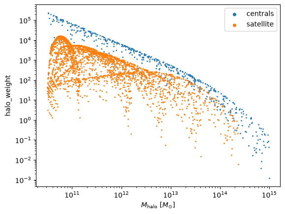
For the weighted lightcone, each halo has multiplicity according to its abundance in the volume

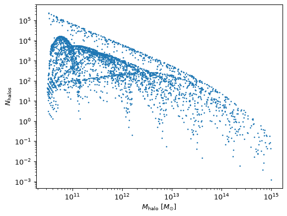
This halo_weight column need to be taken into account when predicting summary statistics from the weighted lightcone. This column stores how each grid point should be weighted in accord with the abundance of halos of the mass and redshift of the grid point.

fig, ax = plt.subplots(1, 1)
__=ax.loglog()
__=ax.scatter(10**lc_data.logmp_obs[lc_data.is_central==1],
              lc_data.halo_weight[lc_data.is_central==1], s=1, label=r'${\rm centrals}$')
__=ax.scatter(10**lc_data.logmp_obs[lc_data.is_central==0],
              lc_data.halo_weight[lc_data.is_central==0], s=1, label=r'${\rm satellite}$')
leg = ax.legend(markerscale=4)
xlabel = ax.set_xlabel(r'$M_{\rm halo}\ [M_{\odot}]$')
ylabel = ax.set_ylabel(r'${\rm halo\_{weight}}$')

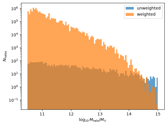
Calculate the halo mass function, accounting for halo weights

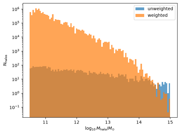
The unweighted version uniformly spans \(\log_{10}M_{\rm halo}\). The weighted version has the expected Schechter-type shape of the HMF.

fig, ax = plt.subplots(1, 1)
yscale = ax.set_yscale('log')
__=ax.hist(lc_data.logmp_obs, bins=100, alpha=0.7, label=r'${\rm unweighted}$')
__=ax.hist(lc_data.logmp_obs, bins=100, weights=lc_data.halo_weight, alpha=0.7, label=r'${\rm weighted}$')
xlabel = ax.set_xlabel(r'$\log_{10}M_{\rm halo}/M_{\odot}$')
ylabel = ax.set_ylabel(r'$N_{\rm halos}$')
leg = ax.legend()

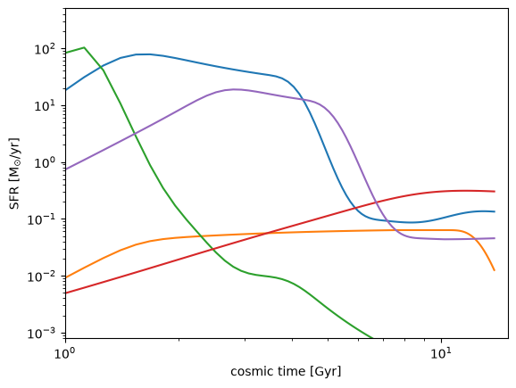
Visually inspect the diversity of SFHs

fig, ax = plt.subplots(1, 1)
yscale = ax.set_yscale('log')
ylim = ax.set_ylim(8e-4, 5e2)
xscale = ax.set_xscale('log')
xlim = ax.set_xlim(1, 15)

n_plot = 5
for i in range(n_plot):
    __=ax.plot(lc_data.t_table, phot_info.sfh_table[i, :])

xlabel = ax.set_xlabel(r'${\rm cosmic\ time\ [Gyr]}$')
ylabel = ax.set_ylabel(r'${\rm SFR\ [M_{\odot}/yr]}$')

Visually inspect the sSFR PDF

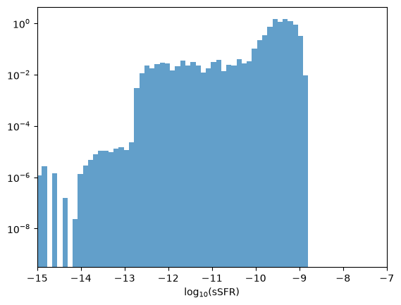
Note that the plot below shows the PDF for all galaxies/halos in the lightcone, without accounting for the weights

fig, ax = plt.subplots(1, 1)
xlim = ax.set_xlim(-15, -7)
yscale = ax.set_yscale('log')
__=ax.hist(phot_info.logssfr_obs, bins=70, alpha=0.7, weights=lc_data.halo_weight, density=True)
xlabel = ax.set_xlabel(r'${\rm log_{10}(sSFR)}$')

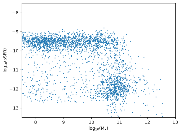
Visually inspect star-forming sequence

fig, ax = plt.subplots(1, 1)
ylim = ax.set_ylim(-13.5, -7.5)
xlim = ax.set_xlim(7.5, 13)
__=ax.scatter(phot_info.logsm_obs, phot_info.logssfr_obs, s=1)
xlabel = ax.set_xlabel(r'${\rm log_{10}(M_{\star})}$')
ylabel = ax.set_ylabel(r'${\rm log_{10}(sSFR)}$')

Plot color-color diagram

Note that the plot below shows the PDF for all galaxies/halos in the lightcone, without accounting for the weights, and without selecting a particular galaxy sample of interest.

fig, ax = plt.subplots(1, 1)

ri = phot_info.obs_mags[:, 2]-phot_info.obs_mags[:, 3]
iz = phot_info.obs_mags[:, 3]-phot_info.obs_mags[:, 4]
__=ax.scatter(iz, ri, s=1)
xlabel = ax.set_xlabel(r'${\rm i-z}$')
ylabel = ax.set_ylabel(r'${\rm r-i}$')

Plot color–redshift relation

Note that the plot below shows the PDF for all galaxies/halos in the lightcone, without accounting for the weights, and without selecting a particular galaxy sample of interest.

fig, ax = plt.subplots(1, 1)

iz = phot_info.obs_mags[:, 3]-phot_info.obs_mags[:, 4]
__=ax.scatter(lc_data.z_obs, iz, s=1)
xlabel = ax.set_xlabel(r'${\rm redshift}$')
ylabel = ax.set_ylabel(r'${\rm i-z}$')

Docs about accounting for the weights, computing high-res SEDs, and more coming soon…