Introduction to soft histograms

This notebook demonstrates the basic principles of using a soft histogram when fitting a model for a probability distribution. We’ll use a one-dimensional Gaussian distribution as our model, and the first thing we’ll do is try to fit the model parameters using a loss function based on a standard histogram. As discussed below, computing standard histograms with hard-edged bins is a non-differentiable calculation, and so our first attempt to fit the model will fail. We’ll then see how using a soft histogram solves the problem.

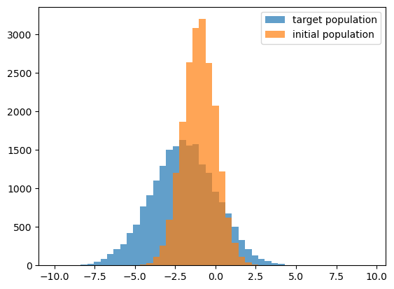
This demo is based on the single_gaussian.py module, which implements a Gaussian model. Let’s start out by using the module to generate some target data with the mc_single_gaussian function, and visually inspect the distributions.

import numpy as np
from matplotlib import pyplot as plt
from jax import random as jran
from jax import numpy as jnp

ran_key = jran.key(0)

import single_gaussian as sg

NBINS = 50
XBOUNDS = (-10.0, 10.0)
XBINS = np.linspace(*XBOUNDS, NBINS)[:-1]


PARAMS_INIT = sg.DEFAULT_PARAMS._replace()
ran_key, init_key = jran.split(ran_key, 2)
XDATA_INIT = sg.mc_single_gaussian(PARAMS_INIT, init_key)

PARAMS_TARGET = sg.DEFAULT_PARAMS._replace(mu=-2.0, sig=2.0)
ran_key, target_key = jran.split(ran_key, 2)
XDATA_TARGET = sg.mc_single_gaussian(PARAMS_TARGET, target_key)

fig, ax = plt.subplots(1, 1)
__=ax.hist(XDATA_TARGET, bins=XBINS,
           alpha=0.7, label=r'target population')
__=ax.hist(XDATA_INIT, bins=XBINS,
           alpha=0.7, label=r'initial population')
leg = ax.legend()

Predicting a histogram from a population

The mc_predict_hard_edged_xhist function is just a wrapper around mc_single_gaussian that first generates target data, and then uses jnp.histogram to bin the data into a predicted histogram.

ran_key, init_key = jran.split(ran_key, 2)
XHIST_INIT = sg.mc_predict_hard_edged_xhist(
    PARAMS_INIT, XBINS, init_key)

ran_key, target_key = jran.split(ran_key, 2)
XHIST_TARGET = sg.mc_predict_hard_edged_xhist(
    PARAMS_TARGET, XBINS, target_key)

Running gradient descent

The hard_edged_xhist_loss_and_grad function is the loss function we will try to minimize with gradient descent. This loss function uses mc_predict_hard_edged_xhist to predict a histogram, and then computes the mean absolute error between the predicted and target histogram. We use jax.value_and_grad to additionally return the gradients of the loss in addition to the value.

The next cell takes 100 steps of gradient descent, where at each step, we take a tiny step down the gradient to update the parameters.

ran_key, loss_key = jran.split(ran_key, 2)
loss_data = XHIST_TARGET, XBINS, loss_key

learn_rate = 0.0005

nsteps = 100
loss_collector = []
p_best = PARAMS_INIT._replace()
for istep in range(nsteps):
    loss, grads = sg.hard_edged_xhist_loss_and_grad(
        p_best, loss_data)
    p_best = sg.param_update(
        p_best, grads, learn_rate)
    loss_collector.append(loss)

Inspect the results

We’ll now inspect the results by plotting the loss curve, and comparing the best-fit histogram to the target.

fig, ax = plt.subplots(1, 1)
xlabel = ax.set_xlabel('step')
ylabel = ax.set_ylabel('log10 loss')
__=ax.plot(np.log10(loss_collector))

ran_key, pred_key = jran.split(ran_key, 2)
xhist_best = sg.mc_predict_hard_edged_xhist(
    p_best, XBINS, pred_key)

fig, ax = plt.subplots(1, 1)
__=ax.plot(XBINS[1:], XHIST_TARGET,
           label='target')
__=ax.plot(XBINS[1:], XHIST_INIT, '--',
           label='initial guess')
__=ax.plot(XBINS[1:], xhist_best, ':',
           label='best fit MC method')
leg = ax.legend()

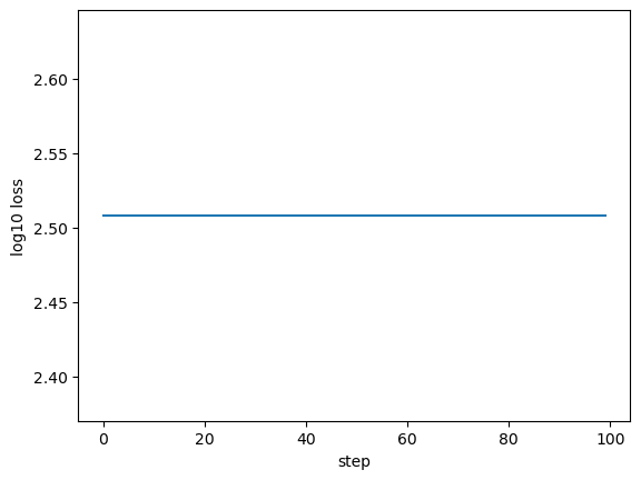
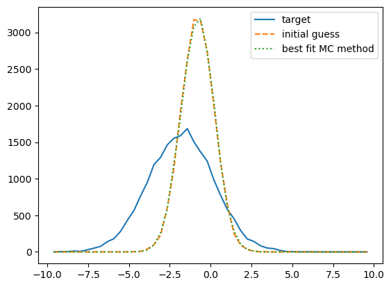
That didn’t work at all - what happened?

It looks like our best-fit histogram didn’t move from the initial histogram. Let’s see how the best-fit points compare to the target and initial points:

gen = zip(p_best._fields, p_best, PARAMS_INIT, PARAMS_TARGET)
for key, val_best, val_init, val_target in gen:
    print(f"Init {key} = {val_init:.2f}")
    print(f"Best {key} = {val_best:.2f}")
    print(f"True {key} = {val_target:.2f}\n")

Init mu = -1.00
Best mu = -1.00
True mu = -2.00

Init sig = 1.00
Best sig = 1.00
True sig = 2.00

Hmmm, the parameters didn’t move at all…

Let’s inspect the gradient

loss_best_mc, grads = sg.hard_edged_xhist_loss_and_grad(
    p_best, loss_data)
print(grads)

GParams(mu=Array(0., dtype=float64), sig=Array(0., dtype=float64))

All the parameters have zero gradients!

That’s why the parameter did not move from its initial position during our gradient descent. The problem comes from trying to differentiate through a histogram with hard-edged bins.

Why don’t hard-edged histograms work with autodiff?

Let’s think about how autodiff works with hard-edged histograms to understand what happened. The way a standard histogram calculation works is that for each bin \(i\), we loop over each point \(x_{\rm j}\) in our dataset, and if the point falls within the boundaries of bin \(i\), we increment our histogram by 1, otherwise we increment by 0. Now consider how the dataset changes with an infinitesimal change to the position of each point, \({\rm d}x\). If \(x_{\rm j}\) is within the bin boundaries, then the perturbed position \(x_{\rm j}+{\rm d}x\) also within the bin boundaries, because the point and the boundary are some finite distance away, and we have only perturbed our point by an infinitesimal amount. The same goes for points outside the bin. The only points with non-zero gradients will be those points that just so happen to fall exactly on the boundary of some bin, a set of measure zero. Thus it makes sense that we get zero-valued gradients for predictions made with hard-edged histograms.

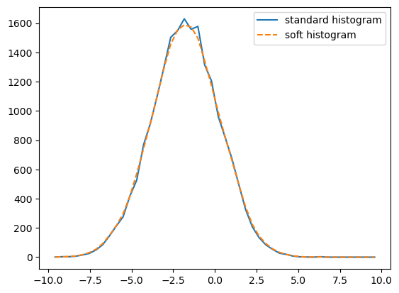
Introducing soft histograms

The solution to this problem is to use soft histograms. In standard histograms, each point in the dataset \(x_{\rm j}\) contributes either 0 or 1 to the result for each bin. In soft histograms, each point contributes a continuously-valued weight, \(w_{\rm j},\) to the result for each bin. Each \(w_{\rm j}\) is computed by integrating a Gaussian kernel across the edges of the bin. For histogram bins with width \({\rm d}x,\) we typically choose a kernel width \(\sigma\lesssim{\rm d}x.\)

There are several soft histogram calculators in diffsky. All of the calculators are written to support N-dimensional data, and so the soft_xhist function in single_gaussian.py just provides some wrapper behavior that reshapes the data and the bins to \({\rm (n, 1)}\).

XHIST_TARGET, __ = jnp.histogram(XDATA_TARGET, bins=XBINS)
XHIST_TARGET_SOFT = sg.soft_xhist(XDATA_TARGET, XBINS)

fig, ax = plt.subplots(1, 1)
__=ax.plot(XBINS[1:], XHIST_TARGET,
           label='standard histogram')
__=ax.plot(XBINS[1:], XHIST_TARGET_SOFT,'--',
           label='soft histogram')
leg = ax.legend()

Running gradient descent with a soft histogram

The next cell takes 100 steps of gradient descent, this time with a loss function based on soft_xhist_loss_and_grad.

ran_key, loss_key = jran.split(ran_key, 2)
loss_data = XHIST_TARGET, XBINS, loss_key

learn_rate = 0.0005

nsteps = 100
soft_loss_collector = []
p_best_soft = PARAMS_INIT._replace()
for istep in range(nsteps):
    loss, grads = sg.soft_xhist_loss_and_grad(
        p_best_soft, loss_data)
    p_best_soft = sg.param_update(
        p_best_soft, grads, learn_rate)
    soft_loss_collector.append(loss)

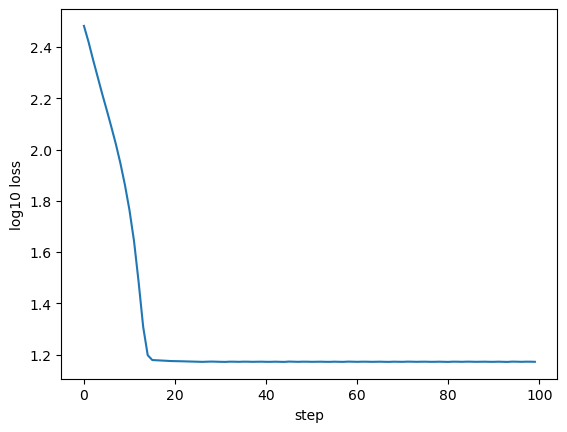
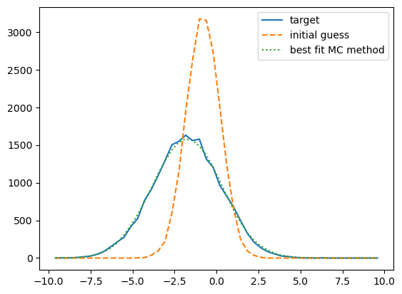
Inspect the results

fig, ax = plt.subplots(1, 1)
xlabel = ax.set_xlabel('step')
ylabel = ax.set_ylabel('log10 loss')
__=ax.plot(np.log10(soft_loss_collector))

ran_key, pred_key = jran.split(ran_key, 2)
xhist_best_soft = sg.mc_predict_soft_xhist(
    p_best_soft, XBINS, pred_key)

fig, ax = plt.subplots(1, 1)
__=ax.plot(XBINS[1:], XHIST_TARGET,
           label='target')
__=ax.plot(XBINS[1:], XHIST_INIT, '--',
           label='initial guess')
__=ax.plot(XBINS[1:], xhist_best_soft, ':',
           label='best fit MC method')

leg = ax.legend()

gen = zip(p_best_soft._fields, p_best_soft, PARAMS_INIT, PARAMS_TARGET)
for key, val_best, val_init, val_target in gen:
    print(f"Init {key} = {val_init:.2f}")
    print(f"Best {key} = {val_best:.2f}")
    print(f"True {key} = {val_target:.2f}\n")

Init mu = -1.00
Best mu = -1.98
True mu = -2.00

Init sig = 1.00
Best sig = 2.02
True sig = 2.00

It worked!

With a soft histogram, when we perturb each point by some infinitesimal amount, the weight of each point also changes infinitesimally, and so we get non-zero gradients.