Fitting a double Gaussian with soft histograms

This notebook shows how to implement a double Gaussian model in JAX, and demonstrates how to optimize the parameters of the model by fitting to soft histograms with gradient descent.

import numpy as np
from matplotlib import pyplot as plt
from jax import random as jran
from jax import numpy as jnp

ran_key = jran.key(0)

Stochastic Monte Carlo predictions

The mc_double_gaussian function generates a sample of 1d data by standard Monte Carlo methods:

1. Draw \(N\) points from the first Gaussian, \(\{\mu_0, \sigma_0\}\)

2. Draw \(N\) points from the second Gaussian, \(\{\mu_1, \sigma_1\}\)

3. Draw \(N\) uniform random numbers, \(u\)

4. If \(f\) is the model parameter controlling the relative height of the two Gaussians, then for points with \(u<f,\) select the random draw from the first Gaussian, otherwise select from the second Gaussian.

This demo is based on the double_gaussian.py module, which implements the above algorithm with the mc_double_gaussian function.

import double_gaussian as dg

NBINS = 50
XBOUNDS = (-5.0, 5.0)
XBINS = np.linspace(*XBOUNDS, NBINS)[:-1]


PARAMS_INIT = dg.DEFAULT_PARAMS._replace()
ran_key, init_key = jran.split(ran_key, 2)
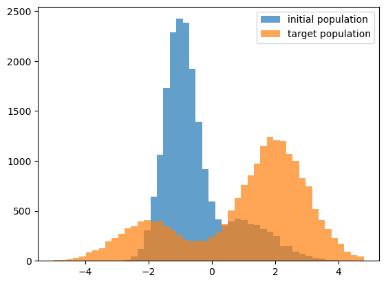
XDATA_INIT = dg.mc_double_gaussian(PARAMS_INIT, init_key)

PARAMS_TARGET = dg.DEFAULT_PARAMS._replace(
    mu0=-2.0, sig0=1.0, mu1=2.0, sig1=1.0, frac0=0.25)
ran_key, target_key = jran.split(ran_key, 2)
XDATA_TARGET = dg.mc_double_gaussian(PARAMS_TARGET, target_key)


fig, ax = plt.subplots(1, 1)
__=ax.hist(XDATA_INIT, bins=XBINS, alpha=0.7, label=r'initial population')
__=ax.hist(XDATA_TARGET, bins=XBINS, alpha=0.7, label=r'target population')
leg = ax.legend()

Predicting a histogram from a population

The predict_soft_xhist_mc function is just a wrapper around mc_double_gaussian that first generates sample data, and then computes a soft histogram of the sample.

ran_key, init_key = jran.split(ran_key, 2)
XHIST_INIT = dg.predict_soft_xhist_mc(PARAMS_INIT, XBINS, init_key)

ran_key, target_key = jran.split(ran_key, 2)
XHIST_TARGET = dg.predict_soft_xhist_mc(PARAMS_TARGET, XBINS, target_key)

Running gradient descent

The mc_mae_loss_and_grad function is the loss function we will try to minimize with gradient descent. This loss function uses predict_soft_xhist_mc to predict a histogram, and then computes the mean absolute error between the predicted and target histogram. We use jax.value_and_grad to additionally return the gradients of the loss in addition to the value.

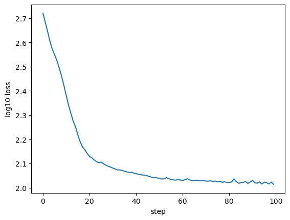
The next cell takes 100 steps of gradient descent, where at each step, we take a tiny step down the gradient to update the parameters.

ran_key, loss_key = jran.split(ran_key, 2)
loss_data = XHIST_TARGET, XBINS, loss_key

learn_rate = 0.001

nsteps = 100

p_best_mc = dg.DEFAULT_PARAMS._replace()
collector_mc = []
for istep in range(nsteps):
    loss, grads = dg.mc_mae_loss_and_grad(p_best_mc, loss_data)
    p_best_mc = dg.param_update(p_best_mc, grads, learn_rate)
    collector_mc.append(loss)

fig, ax = plt.subplots(1, 1)
xlabel = ax.set_xlabel('step')
ylabel = ax.set_ylabel('log10 loss')
__=ax.plot(np.log10(collector_mc))

xhist_best_mc = dg.predict_soft_xhist_mc(p_best_mc, XBINS, target_key)

fig, ax = plt.subplots(1, 1)
__=ax.plot(XBINS[1:], XHIST_TARGET, label='target')
__=ax.plot(XBINS[1:], XHIST_INIT, '--', label='initial guess')
__=ax.plot(XBINS[1:], xhist_best_mc, '--', label='best fit MC method')

leg = ax.legend()

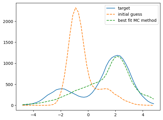
That fit is not so great - what happened?

Let’s see how the best-fit points compare to the target and initial points

for key, val_best, val_init, val_target in zip(p_best_mc._fields, p_best_mc, dg.DEFAULT_PARAMS, PARAMS_TARGET):
    print(f"Init {key} = {val_init:.2f}")
    print(f"Best {key} = {val_best:.2f}")
    print(f"True {key} = {val_target:.2f}\n")

Init mu0 = -1.00
Best mu0 = 1.15
True mu0 = -2.00

Init sig0 = 0.50
Best sig0 = 2.24
True sig0 = 1.00

Init mu1 = 1.00
Best mu1 = 2.15
True mu1 = 2.00

Init sig1 = 1.00
Best sig1 = 0.56
True sig1 = 1.00

Init frac0 = 0.75
Best frac0 = 0.75
True frac0 = 0.25

Hmmm, the frac0 parameter didn’t move

Let’s inspect the gradient

loss_best_mc, grads = dg.mc_mae_loss_and_grad(p_best_mc, loss_data)
print(grads)

DGParams(mu0=Array(-9.37879185, dtype=float64), sig0=Array(11.47065942, dtype=float64), mu1=Array(0.5512829, dtype=float64), sig1=Array(37.95795564, dtype=float64), frac0=Array(0., dtype=float64))

The frac0 parameter has zero gradient!

That’s why the parameter did not move from its initial position during our gradient descent. Since the frac0 parameter has zero gradient, during our gradient descent, the other parameters adjust as best as they can to improve the agreement with the target histogram, and so the loss improves, but the fit still converges to the wrong model since the value of frac0 never departs from its initial value.

Why doesn’t noisy Monte Carlo with autodiff?

For the case of a unimodal Gaussian, it’s no problem at all to fit the model perfectly with predictions based on a noisy MC realization, so what gives?

The frac0 parameter in this model is different from the others: it controls the relative abundance of the two Gaussians, and we use frac0 together with additional draws from a uniform random, so those are some clues why this parameter requires different treatment from the rest.

Let’s first consider why we get non-zero gradients for the other four parameters, \(\{\mu_0, \sigma_0, \mu_1, \sigma_1\}\). Imagine how an infinitesimal change to \(\mu_0\) induces a change to the result of the histogram counts in bin \(i\). As \(\mu_0\) changes, the positions of points \(x_{\rm j}\) drawn from the first Gaussian move, thereby smoothly changing the weights \(w_{\rm j}\) of those points. And so we get non-zero gradients of \(\mu_0\) for our loss function, and similarly for the other three parameters.

Now consider what happens when we perturb the frac0 parameter by some infinitesimal amount, \(\delta f_0\). If our random draw \(u_{\rm j}-f_0\equiv\Delta_{\rm j},\) then since \(\delta f_0<\Delta_{\rm j}\) for an finite difference \(\Delta_{\rm j}\), points to the left and right of \(f_0\) remain to the left and right after the perturbation, and so gradients with respect to \(f_0\) are zero.

What is the solution?

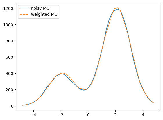
The root problem comes from the stochastic Monte Carlo method we used to choose a particular Gaussian for each point. Instead, we need to compute a \(f_0\)-weighted sum of the soft histogram result of each Gaussian. The predict_soft_xhist_weighted function in double_gaussian.py implements this calculation.

Let’s first observe that the two methods of computing a histogram are equivalent.

XHIST_TARGET = dg.predict_soft_xhist_mc(PARAMS_TARGET, XBINS, target_key)
XHIST_TARGET_WEIGHTED = dg.predict_soft_xhist_weighted(PARAMS_TARGET, XBINS, target_key)

fig, ax = plt.subplots(1, 1)
__=ax.plot(XBINS[1:], XHIST_TARGET, label='noisy MC')
__=ax.plot(XBINS[1:], XHIST_TARGET_WEIGHTED, '--', label='weighted MC')

leg = ax.legend()

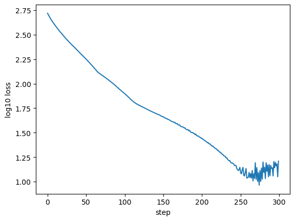
Run gradient descent with weighted soft histograms

params_init = dg.DEFAULT_PARAMS._replace()
loss_init, grads_init = dg.weighted_mae_loss_and_grad(params_init, loss_data)
grads_init

DGParams(mu0=Array(87.82617475, dtype=float64, weak_type=True), sig0=Array(-180.91361185, dtype=float64, weak_type=True), mu1=Array(-71.28411415, dtype=float64, weak_type=True), sig1=Array(31.33326026, dtype=float64, weak_type=True), frac0=Array(542.18128028, dtype=float64, weak_type=True))

learn_rate = 0.00005

nsteps = 300
collector = []
p_best = dg.DEFAULT_PARAMS._replace()
for istep in range(nsteps):
    loss, grads = dg.weighted_mae_loss_and_grad(p_best, loss_data)
    p_best = dg.param_update(p_best, grads, learn_rate)
    collector.append(loss)

fig, ax = plt.subplots(1, 1)
xlabel = ax.set_xlabel('step')
ylabel = ax.set_ylabel('log10 loss')
__=ax.plot(np.log10(collector))

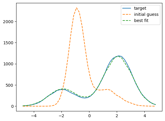
xhist_best = dg.predict_soft_xhist_weighted(p_best, XBINS, target_key)

fig, ax = plt.subplots(1, 1)

__=ax.plot(XBINS[1:], XHIST_TARGET, label='target')
__=ax.plot(XBINS[1:], XHIST_INIT, '--', label='initial guess')
__=ax.plot(XBINS[1:], xhist_best, '--', label='best fit')

leg = ax.legend()

for key, val_best, val_init, val_target in zip(p_best._fields, p_best, dg.DEFAULT_PARAMS, PARAMS_TARGET):
    print(f"Init {key} = {val_init:.2f}")
    print(f"Best {key} = {val_best:.2f}")
    print(f"True {key} = {val_target:.2f}\n")

Init mu0 = -1.00
Best mu0 = -2.00
True mu0 = -2.00

Init sig0 = 0.50
Best sig0 = 1.03
True sig0 = 1.00

Init mu1 = 1.00
Best mu1 = 1.98
True mu1 = 2.00

Init sig1 = 1.00
Best sig1 = 1.01
True sig1 = 1.00

Init frac0 = 0.75
Best frac0 = 0.26
True frac0 = 0.25

It worked!

Upshot: whenever using autodiff to fit models of a multi-modal PDF, we need to compute our soft histograms separately for each mode, and then calculate a probability-weighted sum of the results. Otherwise we get zero-valued gradients for parameters that control the relative abundance of the different modes of the PDF.